Bubble Chart Timeline Excel template

On the off chance that you will utilize attracting apparatuses to make a timetable, there is no restriction to what you can make or how inventive you can get with the outline of your course of events.Bubble Chart Timeline Excel template Be that as it may, in the event that you need something more computerized, you can make a course of events in Excel reasonably effectively, particularly on the off chance that you are utilizing Excel 2013 or later.

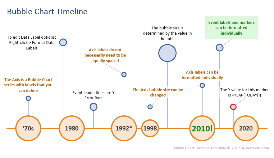
A Bubble Chart in Excel is a generally new kind of XY Chart that uses a third esteem (other than the X and Y facilitates) to characterize the span of the Bubble. Starting with Excel 2013, the information marks for a XY or Bubble Chart arrangement can be characterized by basically choosing a scope of cells that contain the names (while initially you needed to connect singular information names each one in turn). These highlights make it generally simple to make some intriguing courses of events with an air pocket graph.

Bubble Chart Timeline Template

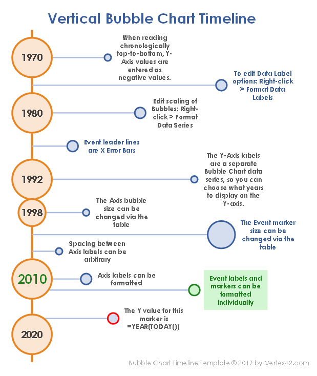
Vertical Bubble Chart Timeline

Create a Bubble Chart Timeline in Excel

You can take after the means beneath to make your own course of events starting with no outside help. The directions are for making a level course of events. On the off chance that you need to make a vertical course of events, you can take after the means substituting the Y-hub for the X-pivot. Additionally, in the event that you need the vertical course of events to peruse sequentially through and through, the Y-values should be negative. The layout above can demonstrate to you how that functions.

Watch the How To Video!

Stage 1: CREATE THE AXIS BUBBLE CHART SERIES 

Something individuals regularly whine about while making courses of events in Excel is the trouble of tweaking the names for the timetable hub. 

The strategy I'm displaying here overlays a Bubble Chart information arrangement over the highest point of the ordinary X-hub.Bubble Chart Timeline Excel template This enables you to control the separating between the pivot marks AND to include whatever names you need. You don't have to utilize numeric names on the off chance that you would prefer not to.

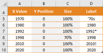
Set up the AXIS information table (like the picture to one side) 

Select cells A5:C10 and go to the Insert tab and pick the XY Bubble diagram compose 

Right-tap on an air pocket and select Format Data Series to organize it the way you need

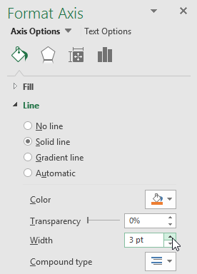
Stage 2: FORMAT THE X-AXIS LINE AND REMOVE LABELS 

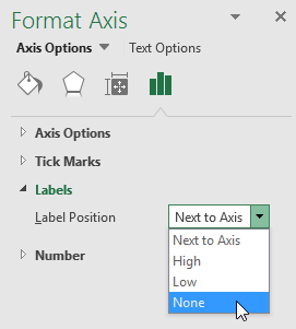
Right-tap on the names for the X-hub and select Format Axis 

For the Label Position, select None 

For the Line arrange alternatives, pick the shading you need and increment the line width

Remove Axis Labels

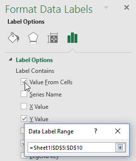
STEP 3: CREATE CUSTOM AXIS LABELS WITHIN THE AXIS BUBBLES

Right-tap on the hub bubbles and select Add Data Labels (these will appear as little marks that you won't not see at first) 

Right-tap on the hub bubbles again and select Format Data Labels 

Check the "Esteem From Cells" alternative and select the range from your Axis Labels table 

Uncheck the Y Value and pick Center for the Label Position 

Increment the text dimension and alter the textual style design as wanted. You can choose and design every datum mark independently on the off chance that you need to (like the 2010! mark in this case)

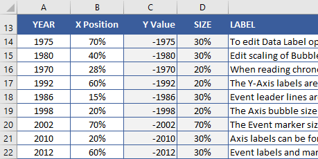
STEP 4: ADD A NEW DATA SERIES FOR THE TIMELINE EVENTS

The subsequent stage is to include the course of events occasions. We can utilize a different information table for posting the occasions.Bubble Chart Timeline Excel template I have discovered that I regularly need to enter the date or year for an occasion uniquely in contrast to what the esteem should be for the outline. 

For instance, while making a vertical timetable with occasions indicated sequentially start to finish, the Y-values should be negative. Yet, I need to enter the years as ordinary positive numbers. In this way, I have a different section for the Y-esteem which for this situation is a basic equation like =-YEAR

To make the information arrangement for the course of events occasions ... 

Right-tap on the graph and pick Select Data 

Tap on Add to include another information arrangement. Name it something like "Occasions" and pick the YEAR for the X Values, the Y Position for the Y Values, and the Size for the Size esteems. On the off chance that you are making a vertical timetable, the X and Y esteems will be swapped. 

After the air pocket markers for your occasions appear in your diagram,Bubble Chart Timeline Excel template right-tap on an air pocket and select Format Data Series to pick the hues for the line and fill for the air pocket markers. 

Note: If the markers for your new information arrangement don't appear in your diagram, ensure your even and vertical pivot limits are set to Automatic or ensure that your information really fits inside the hub limits. 

To alter the limits for the tomahawks, right-tap on the pivot and select Format Axis. 

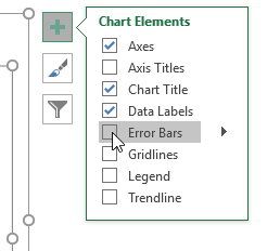
Stage 5: ADD LEADER LINES AS Y ERROR BARS 

Pioneer lines from the course of events occasions to the timetable pivot can be made by adding vertical mistake bars to the timetable occasion markers. To do that 

Tap on a rise in the occasion arrangement then the + image and select Error Bars (see the picture on the right)

 

Select one of the X-blunder bars and press Delete to evacuate them 

Right-tap on the Y-mistake bars and select Format Error Bars 

Pick Minus for the bearing, No Cap for the end style, and Percentage = 100% for the blunder sum. 

In the Line alternatives (under the pail), you can arrange the mistake bar lines to be the shading and width that you need. 

For a vertical course of events, swap "X" and "Y" in stages 2 and 3 (expelling the Y-blunder bars and modifying the X-mistake bars). 

Stage 6: ADD EVENT LABELS 

Right-tap on the occasion arrangement and select Add Data Labels 

Right-click again on the occasion arrangement and select Format Data Labels 

Like before with the pivot, pick Value From Cells at that point select the scope of marks from your table. 

Pick Above for the Label Position, and uncheck the Y Value. 

On the off chance that you need to show the X-Axis esteem in the information mark, you can check the X Value alternative. 

For the information marks, I like utilizing a strong white fill set to around 25% straightforwardness, so that if the names cover the pioneer lines, you can at present faintly observe the pioneer line behind the name. 

Stage 7: MODIFY TIMELINE EVENT POSITIONS TO GET EVERYTHING TO FIT 

The Y Position esteems in the table are utilized to position the markers so the names don't cover. That is frequently the greatest test while making a course of events. In the event that you have a ton of occasions packed into a brief period, you may need to get innovative or you may need to think about utilizing a variable-scale hub (where the separation between the Axis Labels isn't correct). 

Right-tap on the Y-pivot and set the Maximum bound to 1 and the Minimum bound to - 0.2. The Y Positions in the Events table can be entered as a %, speaking to a separation in the vicinity of 0 and 1 (1=100%). 

In the wake of changing the Y-hub, you can erase it by choosing the pivot and squeezing Delete. 

Notwithstanding changing the vertical position of the markers, you can drag singular names to fit them as required. 

Peculiar EXCEL BUG: LABELS NOT SHOWING UP? 

On the off chance that you spare the document with some clear columns in your information table, when you open the record later you may find that the marks don't appear in the outline when you include the names into the clear lines. On the off chance that this happens, I've discovered that I can erase the columns where the names aren't working and after that embed new lines and re-enter the information (or broaden the table down utilizing the drag handle). 

Another work-around: In the Format Data Labels window (1) Click on the Reset Label Text catch, (2) UNcheck the Value From Cells alternative, (3) Re-Check the Value From Cells choice. 

References 

Make a Timeline in Excel at Vertex42.com - The utilization of blunder bars for pioneer lines and information marks connected to an information table was first displayed by Jon Wittwer of Vertex42 in this article Sep 2, 2005. 

Exhibit your information in an air pocket graph at support.office.com - This doesn't discuss courses of events, however it demonstrates to make an essential air pocket diagram in Excel.