Vertical Timeline Excel Template

A vertical course of events can be made in Excel utilizing a X-Y Scatter Plot, Data Labels, and Error Bars for the pioneer lines.Vertical Timeline Excel Template This procedure was spearheaded by Vertex42 in the first Timeline Template in 2005. More up to date forms of Excel, starting with Excel 2013, incorporate a component that makes making timetables without any preparation considerably less demanding than it used to be. Keep perusing underneath to figure out how to make a vertical course of events, or download the format to get a head begin.

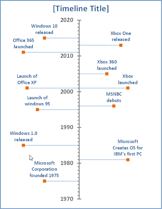
Vertical Timeline

PRINTING THE TIMELINE

When printing an outline in Excel, you can choose the diagram and press Ctrl+p to print the graph fit to a solitary page. In any case, if your course of events is long or you need to print the graph over various pages, select the scope of cells behind your diagram and print that scope of cells. 

You can utilize custom scaling by means of the print settings to print over numerous pages. You'll need to do some cutting and taping a short time later, however in the event that you have the tolerance to do that, it's a sensible method to make a publication estimate course of events to show in a classroom or meeting.

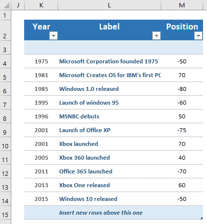
Stage 1: CREATE THE DATA TABLE 

You'll require a segment for the year, portrayal, and the level position. The picture beneath demonstrates the case utilized as a part of the layout.

When utilizing a X-Y Scatter Plot, it isn't important to sort the occasions in the table by date. It might be advantageous to arrange your information table as an Excel table. 

Stage 2: CREATE THE X-Y SCATTER PLOT 

Select the Year section and the Position segment 

Go to Home > Insert > Charts and embed a Scatter Chart 

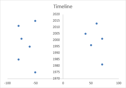
After this progression, your course of events will show up as a flat timetable. You now need to switch the x-hub and y-hub to make the course of events vertical.Vertical Timeline Excel Template You can do that by altering the diagram information source, however you can likewise choose the information arrangement inside the graph and swap the references specifically in the equation bar. 

=SERIES("Timeline",Sheet1!$M$3:$M$15,Sheet1!$K$3:$K$15,1) 

Tap on the gridlines and press Delete to tidy up the graph. Now, your timetable may resemble this:

Stage 3: CREATE LEADER LINES AS HORIZONTAL ERROR BARS 

Pioneer lines interfacing the markers to the pivot can be made by including even mistake bars.Vertical Timeline Excel Template To include them, tap the graph and check the "Mistake Bars" confine the rundown of Chart Elements, at that point take after these means:

Select one of the vertical mistake bars and press Delete to expel them 

Right-tap on the level mistake bars and select Format Error Bars 

Pick Minus for the bearing, No Cap for the end style, and Percentage = 100% for the Error Amount. 

Arrangement the shading, width, dash compose, and different parts of the pioneer lines 

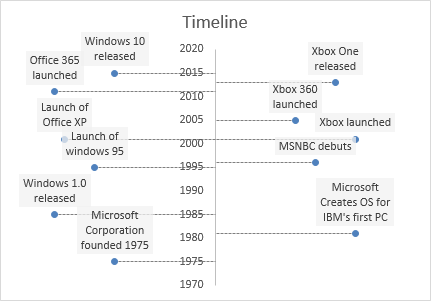
Stage 4: ADD EVENTS AS DATA LABELS 

Right-tap on the information arrangement and select Add Data Labels 

Right-click again on the information arrangement and select Format Data Labels 

Pick Value From Cells at that point select the section names from your table. 

Pick Above for the Label Position, and uncheck the Y Value. 

For the information marks, utilize a strong shading fill set to around 25% straightforwardness. This permits you faintly observe through the mark on the off chance that it covers different occasions or pioneer lines. 

Now, the graph will resemble the case beneath.

Stage 5: FORMAT AND POSITION 

Now, all that is left is to organize your graph how you need it and alter the position esteems for every one of the occasions to get everything to fit pleasantly. 

Arrangement the vertical pivot (shading, min/max esteems, number configuration, and so on.) by right-tapping on the hub and choosing Format Axis. 

In the event that you need the vertical hub on the left and all occasions on the right, set the level hub Minimum incentive to 0 and alter the Positions in the table to be all positive numbers. 

When working with the situating of the occasions, I think that its most straightforward to set the Min/Max limits for the level hub to - 110 and 110 (or 0 and 110). 

You can design singular markers and information names by first choosing an individual information point or name. 

To show the year as 15,000 BC or 2,000 AD, you can utilize a custom number arrangement: 

Right-tap on the x-hub and select "Arrangement Axis..." 

In the Format Axis discourse box, go to Number, select Custom from the class list and enter the accompanying in the Format Code box: #,##0 "AD";#,##0 "BC" 

Abnormal EXCEL BUG: LABELS NOT SHOWING UP? 

In the event that you spare the document with some clear columns in your information table, when you open the record later you may find that the marks don't appear Vertical Timeline Excel Template in the outline when you include the names into the clear lines. On the off chance that this happens, I've discovered that I can erase the columns where the names aren't working and afterward embed new lines and re-enter the information (or broaden the table down utilizing the drag handle). 

Another work-around: In the Format Data Labels window (1) Click on the Reset Label Text catch, (2) Uncheck the Value From Cells choice, (3) Re-Check the Value From Cells choice.